

Bouncing Balls
Run a basic, explosion or entropy simulation; or create create your own.
The amount of physical phenomenon that can be visualised through mere "bouncing balls" is staggering.
Once quantum computers are able to maintain numerous qubits with high stability, we will be able to simulate atomic and molecular behaviour in great depth. This should lead to advancements in areas such as drug research and material science.
Whilst we're waiting, I thought I'd go about trying to simulate particle collision behaviour on a classical computer.
This was achieved in an HTML Canvas Element which I interfaced with directly through the JavaScript language.
The remainder of this post will discuss the implementation of this simuation. There are links at the top to a couple of pre-constructed simulations alongside a link to build your own.
The code for this project is here on GitHub.
In terms of data structures, each ball is stored with basic properties: a position vector, a velocity vector and a radius. Since all balls have identical artificial density, the mass of each ball is proportional to its radius so would be reduntant to store.
The verticies of the rectangular obstacles (hereafter referred to as "bollards") are represented through position vectors.
These data structures are randomly populated at run time based on data that is encoded in the URI of the webpage. [To run the simulation, a link which includes the correct encoded data must be generated by the world builder page, builder.html, that is linked at the top of this post.]
After initialisations, the main event loop is entered with window.requestAnimationFrame.
At the end of the event loop function, the function recursively requests itself for the next animation frame too. This gives the browser time to process user events, but avoids any explicit delays in the code to ensure the smoothest rendering. We are also passed a timestamp which allows us to compute a time delta from the previous frame. This is then encorporated into our equations of motion.
We can now concern ourselves with the core of the code. Which is coordinated from this main loop.
We consider the following tasks,
- applying the acceleration due to gravity to each ball;
- processing any ball~wall collisoins;
- processing any ball~ball collisions;
- processing any ball~bollard collisions;
- incrementing the ball position vectors by their velocity vectors;
- re-drawing the canvas.
Having broken down the code, the main event loop, seen below, is quite readable.
/******************
      MAIN LOOP
*******************/

function update(time_ms){
    time_delta_s = last_time_ms ? (time_ms - last_time_ms) / 1000 : 0;
    last_time_ms = time_ms;

    apply_gravity();

    wall_collisions();
    ball_collisions();
    bollard_collisions();

    update_ball_positions();

    clear_screen();
    draw_screen();

    requestAnimationFrame(update);
}
I do not wish to step through the remainer of the code line-by-line. Instead, I will cast a more asbstract overview of the implementation.
Firstly, applying gravity is simple. Acceleration is the rate of change of velocity, dv/dt = a. Integrating this, we have v = at + c. Letting v = u at t = 0 we derive one of the five equations of motion: v = u + at. So we simply need to increment the y-component of each ball's velocity by gravity scaled by the time delta.
As for collisions, wall collision is simple, but ball and bollard collision handling is considereably more challenging.
In general, collision processing can be broken down into two (or three if your include assigning velocities) stages:
- detecting a collision;
- calculating velocities.
We now see how the case of the wall is simple: if the orthogonal distance from the ball's centre to a wall is less than its radius, we invert the respective velocity component by multiplying it by -1.
Progressing to the easier of the two remaining cases, the ball~bollard collision, we see the computation becomes more difficult.
In this case, detection is carried out by considering the perpendicular (shortest) distance between the ball and the side of the rectangle that is currently being evaluated - if it is less than the ball's radius, then we may have a collision. We must additionally check that the ball is within the two other parrallel sides of the rectangle. This is computed by checking whether the sign of the distance between the ball and each of these two sides match (this works since the verticies of the rectange are cyclically numbered).
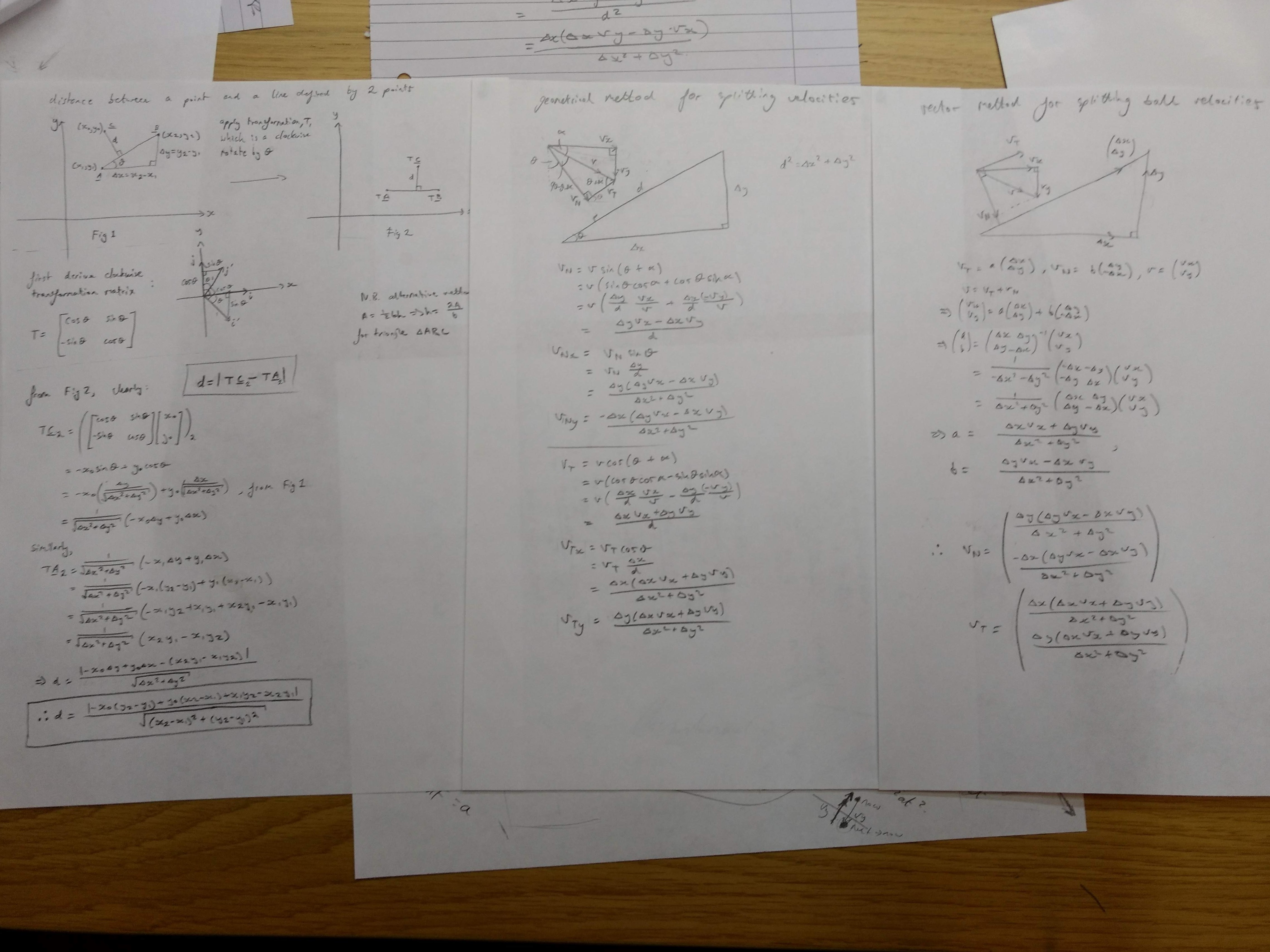
How is this point-line distance calculated though? Well on reflection, I looked up the proper way to do so on Wikipedia, but that was after I had discovered my own long-winded method. I used a matrix to rotate all three points so that the two points on the line lied horizontally. This meant that the distance could then be read off directly as the difference between the y-coordinates of the transformed point and one of the transformed line points. These calculations are seen belwo.
Now we must consider step (2). In order to calculate the resulting velocity vector, we must resolve the ball's current velocity vector into components that are tangent and normal to the line of least distance between the ball and the line. We can then simply invert the normal component and then combine the two vectors back together.
And how do we resolve the velocity vector? I found that you can use plain geometry or, again, a little linear algebra. These calculations, along with my way of calculating point-line distance, are seen below.
And that completes ball~bollard collisions.
In the case of ball~ball collisions, detection is done by seeing if the magnitude of the centre-centre distance, calculated by pythagoras, is less than the sum of the radii.
We then follow a similar thought process to that of the ball~bollard collisions resolving the two ball velocities into normal and tangent components. However we now use ideas of energy and momentum to calculate the final normal component before combining the vectors back together again.
To resolve the velocities, the calculations are much the same as before, so I will not post those.
The important step here is how we calculate the final normal velocities of the two balls given their initial velocities and their masses. Lacking much knowledge further than momentum is mass times velocity (p = mv) and that "momentum is conserved" (i.e. m1u1 + m2u2 = m1v1 + m2v2), I needed some assistance working out the final normal velocities in an elastic (a special type of collision in which kinetic energy is conserved) collision. I came across this resource that derived the 1d equation I desired. And in essence, that completes ball~ball collisions; we just combine the modified normal and unchagned tangent vectors and assign them back to their respective balls.
That's pretty much all. As previously stated, the world builder page allows for the design of a simulation which is encoded in a URI query parameter in the form of a link - allowing you to make your own simulations. On the other hand, just take a look at the few I made myself which are linked at the top of the post.